Using the Code
Overview
SIMBA is implemented entirely in Python, prioritizing code clarity while achieving acceptable performance through targeted optimization. The code is structured into several modules that handle distinct aspects of the chemical modelling. This modular design improves maintainability by separating distinct functionalities, facilitates testing by isolating components, and allows users to extend individual components without affecting the rest of the codebase.
The core data structures are implemented using Python’s dataclass framework, which provides a concise way to create classes focused on data storage with built-in validation. The primary dataclasses are:
Species: Contains arrays of abundances, masses, and charges for chemical species, alongside their namesReactions: Stores reaction networks including reactants, products, rate coefficient parameters, and temperature limitsGasandDust: Hold physical properties such as temperatures and densities for each phaseEnvironment: Contains parameters describing the local conditions like radiation field strength, extinction, and ionization ratesParameters: Stores simulation settings and physical constants
Each dataclass includes validation methods that ensure physical constraints are met (e.g., positive temperatures, valid abundance ranges) and type checking.
Rate coefficients are calculated using a type-based classification system that is deliberately compatible with the established DALI code (Bruderer et al. 2012, 2013). By adopting the same reaction type identifiers, SIMBA can seamlessly use chemical networks developed for DALI without requiring reformatting or conversion. This design choice facilitates network validation and comparison of results between codes, and a detailed benchmarking of SIMBA against DALI is presented in our code overview paper. While the code currently reads networks in the DALI format, the modular structure allows users to easily implement additional parsers for other network formats, provided they map the reactions to the appropriate type identifiers. An example network (first presented in Keyte et al. 2023) is provided with the code.
The core solver is implemented in the Simba class, which manages the chemical network integration. This class employs the scipy.integrate.solve_ivp routine with the backward differentiation formula (BDF) method, which is particularly suitable for the stiff systems characteristic of astrochemical networks. Performance-critical numerical routines are optimized using numba just-in-time compilation. This includes the calculation of chemical derivatives and the Jacobian matrix. The derivatives function computes formation and destruction rates for each species, while the Jacobian calculation is optimized for the typically sparse structure of chemical networks, where most species interact with only a small subset of the total network.
Self-shielding calculations are handled by a dedicated module that pre-loads tabulated shielding factors during initialization. For \(\small{\text{CO}}\) and \(\small{\text{N}}_2\), this module implements interpolation routines that operate on the tabulated data, while \(\small{\text{H}}_2\) and \(\small{\text{C}}\) self-shielding are computed using their analytical approximations.
The code also includes comprehensive analysis and visualization capabilities through a dedicated analysis module and graphical user interface. This provides plotting functions for species abundances and reaction rates over time, as well as tools for investigating chemical pathways and network properties. Data can also be exported in standard formats for further analysis.
Input File
SIMBA reads its configuration from a simple text-based input file (.dat) that defines the physical conditions, environmental parameters, and runtime settings for the simulation.
Example Input
Here’s a representative input file with typical values:
# SIMBA Input File

n_gas          = 1.190e+08
n_dust         = 2.498e+05
t_gas          = 1830.8
t_dust         = 148.0
gtd            = 4.763e+02
Av             = 3.136e-01
G_0            = 6.419e+04
Zeta_X         = 5.626e-14
h2_col         = 5.489e+18
self_shielding = True
column         = True
Zeta_CR        = 5e-17
pah_ism        = 0.1
t_chem         = 1e6
network        = 'chemical_network.dat'
Parameter Definitions
Parameter |
Description |
Units |
|---|---|---|
|
Number density of gas |
cm³ |
|
Number density of dust grains |
cm³ |
|
Gas temperature |
K |
|
Dust grain temperature |
K |
|
Gas-to-dust number density ratio |
dimensionless |
|
Visual extinction |
mag |
|
Local FUV field strength in Draine units |
~2.7 x 10⁻³ erg s⁻¹ cm⁻² |
|
X-ray ionization rate |
s⁻¹ |
|
H₂ column density |
cm⁻² |
|
Enable self-shielding calculations for H₂, N₂, CO, and C |
boolean |
|
Use user-specified H₂ column density ( |
boolean |
|
Cosmic ray ionization rate |
s⁻¹ |
|
PAH abundance relative to ISM value |
dimensionless |
|
Chemical evolution time |
years |
|
Path to chemical network definition file |
string |
Creating an Input File
You can generate a template input file using the built-in helper function:
import simba_chem as simba
simba.create_input("path/to/save/input_file.dat")    # then modify with your specific parameters
Chemical Network
The chemical network file specifies the complete set of chemical species, reactions, and rate coefficients that drive the chemical evolution in SIMBA. By design, SIMBA is configured to read chemical networks with identical format to that of the widely-used DALI thermochemical code, enabling direct comparison with published results and facilitating ease-of-use.
Default Network
A standard chemical network is included with the installation (originally presented in Keyte et al. 2023). You can create a copy of this network using the helper function:
import simba_chem as simba
simba.create_network("directory/to/save/network/")
The copied network file can then be modified to include additional reactions, adjusted for specific chemical conditions, or used as a template for creating a new network.
The file follows a structured format with three main sections:
A list of elements that form the basic building blocks
A comprehensive list of atomic and molecular species, including their properties
A detailed list of chemical reactions and their rate coefficients
Correct formatting must be maintained throughout the file, as parsing errors can occur even with minor deviations. The expected structure is detailed in the sections below.
Network File Format
Elements Section
! n_elements
10
! LIST OF ELEMENTS
H
He
C
N
O
Mg
Si
S
Fe
Pa
Species Section
! n_species
135
! LIST OF SPECIES
!             < Initial     amu chr H  He C  N  O  Mg Si S  Fe Pa
H               1.000e+00     1  0  1  0  0  0  0  0  0  0  0  0
He              7.590e-02     4  0  0  1  0  0  0  0  0  0  0  0
C               1.000e-05    12  0  0  0  1  0  0  0  0  0  0  0
N               2.140e-05    14  0  0  0  0  1  0  0  0  0  0  0
O               2.000e-05    16  0  0  0  0  0  1  0  0  0  0  0
...
Each species entry contains:
Species name
Initial abundance
Molecular mass (amu)
Charge (0, +1, -1 etc)
Element composition (counts of each element)
⚠️ Important notes:
• PAHs are treated as a separate element in the species list (‘Pa’)
• The PAH abundance should be set to the ISM value ~ 4.17e-8
• The desired PAH abundance is then set using thepah_ismparameter in the Input File
• Ice-phase species are preceded with ‘J’ (eg. ice-phase ‘CO’ is denoted ‘JCO’)
• Vibrationally excited H₂ is denoted ‘H2*’
Reactions Section
! n_reactions
1875
!
!e1           e2            e3            p1            p2            p3            p4            p5               nr  type  a            b            c            temp_min     temp_max   pd-data
H             CH                          C             H2                                                          16  20   1.310e-10    0.000e+00    8.000e+01    0.000e+00    2.000e+03  ---------
H             CH2                         CH            H2                                                          17  20   6.640e-11    0.000e+00    0.000e+00    0.000e+00    2.500e+03  ---------
H             NH                          N             H2                                                          18  20   1.730e-11    5.000e-01    2.400e+03    0.000e+00    3.000e+02  ---------
H             CH3                         CH2           H2                                                          19  20   1.000e-10    0.000e+00    7.600e+03    0.000e+00    2.500e+03  ---------
H             NH2                         NH            H2                                                          20  20   5.250e-12    7.900e-01    2.200e+03    0.000e+00   -1.100e+03  ---------
H             NH2                         NH            H2                                                          21  20   1.050e-10    0.000e+00    4.450e+03    1.100e+03    3.000e+03  ---------
...
Each reaction entry contains:
Field |
Description |
|---|---|
e1-e3 |
Reactant species (up to 3) |
p1-p5 |
Product species (up to 5) |
nr |
Reaction number |
type |
Reaction type code |
a |
Rate coefficient \(\alpha\) |
b |
Rate coefficient \(\beta\) |
c |
Rate coefficient \(\gamma\) |
temp_min |
Minimum valid temperature (K) |
temp_max |
Maximum valid temperature (K) |
pd-data |
Photodissociation data (not currently used) |
Reaction Types
The network includes several categories of reactions, indicated by the type code:
Surface Chemistry (10-12)
10: H₂ formation on grains
11: Hydrogenation
12: Photodesorption
Gas Phase (20-22)
20: Standard gas-phase reactions
21: Temperature-limited reactions (no extrapolation)
22: Temperature-bounded reactions (switched off outside range)
Photochemistry (30-33)
30: Standard photodissociation
31: H₂ photodissociation with self-shielding
32: CO photodissociation with self-shielding
33: C photoionization with self-shielding
38: N₂ photodissociation with self-shielding
Cosmic Ray Chemistry (40-43)
40: Direct cosmic ray ionization
41: Cosmic ray induced FUV reactions
42: Cosmic ray induced CO dissociation
43: Cosmic ray induced He decay
X-Ray Chemistry (60-62)
60: X-ray secondary ionization of H
61: X-ray secondary ionization of H₂
62: X-ray secondary ionization of other molecules
PAH Chemistry (70-72)
70: PAH photoelectron production
71: PAH charge exchange/recombination
72: Mass-scaled PAH reactions
Grain Chemistry (80-81)
80: Thermal desorption
81: Freeze-out
H₂* Chemistry (90-92)
90: H₂ excitation
91: H₂* de-excitation
92: H₂* reactions
⚠️ Important note:
• Self-shielding of CO isotopologues is not currently implemented
Alternative Network Formats
SIMBA is currently configured to only read DALI-format network files. However, support for alternative formats can be added by modifying the code:
Create a Python function that reads your network file and returns the following arrays:
def read_custom_network(filename):
    # Your parsing code here
    return (n_elements, elements_name,
            n_species, species_name, species_abu,
            species_mass, species_charge,
            n_reactions, reactions_educts, reactions_products,
            reactions_reaction_id, reactions_itype,
            reactions_a, reactions_b, reactions_c,
            reactions_temp_min, reactions_temp_max,
            reactions_pd_data)
Replace the
read_chemnetfunction in thesimba_helpersmodule with your custom functionEnsure your network follows these requirements:
Uses the same reaction type IDs as described in this documentation
Maintains consistent array shapes and data types
Includes all required fields for species and reactions
Running the Code
Single-point (0D) models
A single-point model can be run easily with just a few lines of code. See the Quick Start guide for details.
1D (+higher dimension) models
SIMBA can be easily extended from single-point (0D) to multi-dimensional models by creating a grid of input parameters and running individual instances for each grid cell. This approach allows you to efficiently model chemical evolution across spatial gradients in density, temperature, radiation field strength, or any other environmental parameter.
Most astrochemical modeling codes implement “static” models, where each grid cell is initialized with identical starting abundances and evolved to the same chemical age. The only differences between cells are the physical parameters (density, temperature, radiation field, etc.). SIMBA readily supports this conventional approach, an example of which is presented in Keyte & Ran (2025).
SIMBA also offers additional flexibility for modeling systems with time-varying physical conditions. Unlike static models, this approach allows you to track chemical evolution through dynamically changing environments by:
Running a model with initial physical conditions
Using the final chemical state as the initial state for the next model
Updating physical parameters for the next time step
Repeating to follow the chemical evolution through the changing environment
This capability is particularly valuable for modeling systems undergoing significant physical changes, such as protoplanetary disks with evolving temperature/density profiles, gas parcels moving through varying radiation environments etc. A simple dynamical 1D model is presented in our code overview paper.
Analysis Tools
The Analysis module provides simple plotting routines for visualizing results, including:
Abundances vs. Time
Reaction Rates vs. Time
Dashboard showing key diagnositics
First, initialize the model, run the simulation, and instantiate the Analysis module:
import simba_chem as simba
network = simba.Simba()                          # create an instance of SIMBA
network.init_simba("path/to/input_file.dat")     # initialise the network
network.solve_network()                          # run the solver
analysis = simba.Analysis(network)               # access analysis
All analysis functions return the underlying Matplotlib Figure and Axes objects, allowing users to further customize or save the plots as needed. Figures are only displayed automatically when show=True, ensuring consistent behavior in scripts, notebooks, and non-interactive environments.
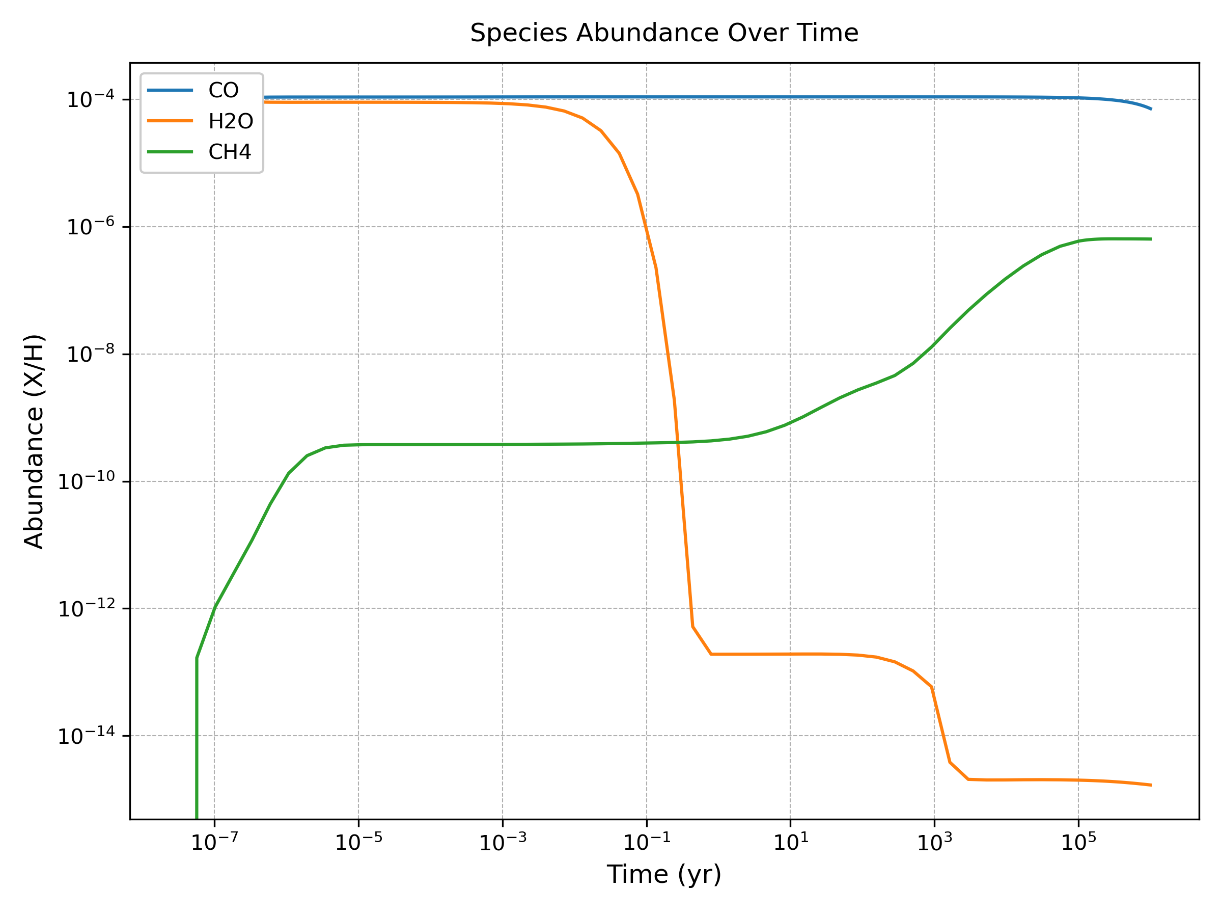
Abundances vs. Time
The plot_abundance() method generates time-evolution plots for specified chemical species:
analysis.plot_abundance(['CO', 'H2O', 'CH4'], show=True)
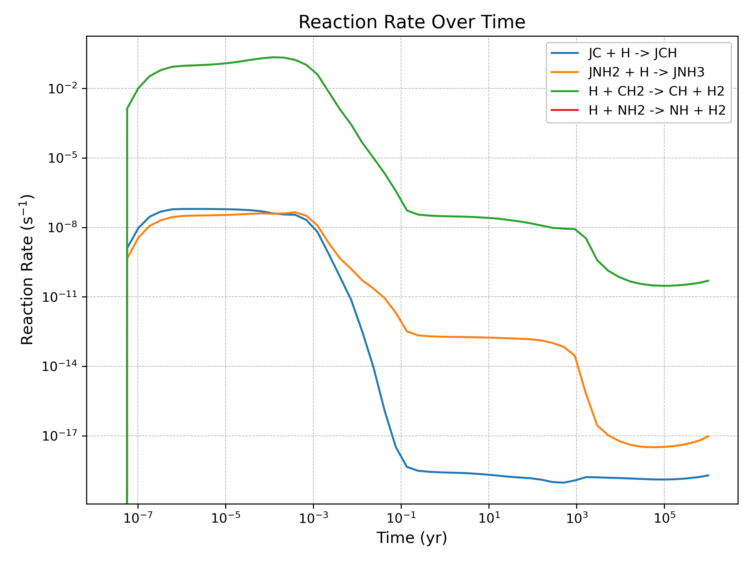
Reaction rates vs. Time
The plot_reaction_rate() method generates time-evolution plots for individual reaction rates, taking in a list of reaction IDs (as defined in the chemical network)
analysis.plot_reaction_rate([1, 7, 18, 22], show=True)
It can sometimes be useful to plot all the major formation and destruction reactions for a particular species. This can easily be done with a short code, eg:
fig, ax = plt.subplots(1,2, figsize=(15,6), sharey=True)

species = 'CO'

rate_threshold = 1e-14  # only show rates above some threshold

# Find reaction data
species_formation   = []
species_destruction = []

for i in range(0, network.parameters.n_reactions):
    if species in network.reactions.products[i]:
        species_formation.append(i)
    if species in network.reactions.educts[i]:
        species_destruction.append(i)

# Plot formation rates
for i in species_formation:
    if np.max(result['rates'][:,i]) > rate_threshold:
        ax[0].plot(result['time']/network.parameters.yr_sec, result['rates'][:,i], label=result['reaction_labels'][i])

# Plot destruction rates
for i in species_destruction:
    if np.max(result['rates'][:,i]) > rate_threshold:
        ax[1].plot(result['time']/network.parameters.yr_sec, result['rates'][:,i], label=result['reaction_labels'][i])

for j in range(0,2):
    ax[j].set_xscale('log')
    ax[j].set_yscale('log')
    ax[j].legend()

plt.tight_layout()
plt.show()
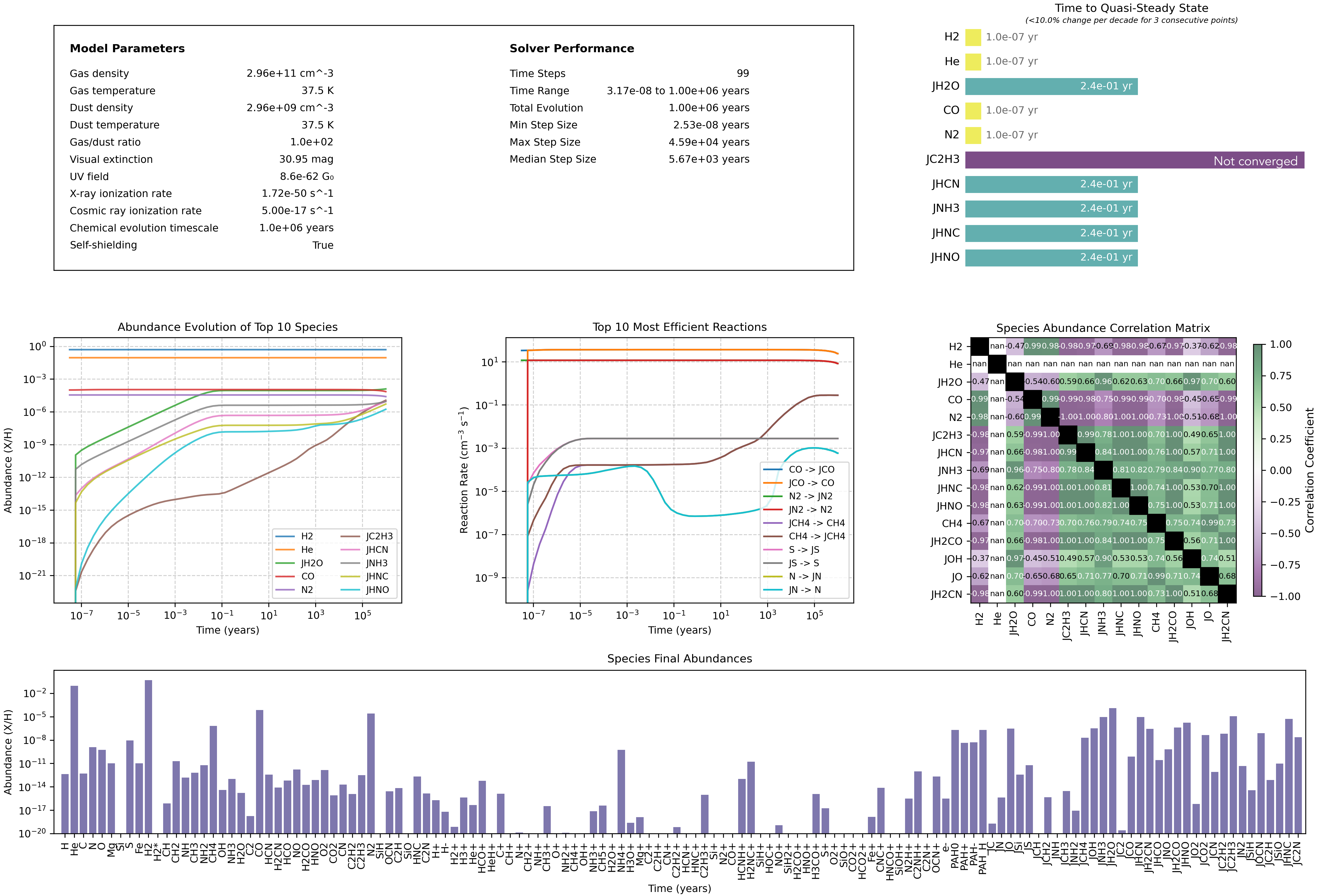
Dashboard
NOTE: The Dashboard tool is a work-in-progress! Please use at your own risk!
The dashboard displays model parameters and other useful diagnostic plots including:
Solver statistics
Quasi steady-states timescales (top 10 most abundant species)
Abundances vs. time (top 10 most abundant species)
Reaction rates vs. time (top 10 most efficient reactions)
Species correlation matrix
Final abundances of all species
analysis.plot_dashboard()
Additional tools
Additional analysis tools (eg. interactive plots, network path analysis) are available in the GUI. Future versions of the code will also include these in the Analysis module.
Export data
Abundance data can be exported to .csv format using the helper function in the Analysis module:
# Export abundances to CSV
analysis = simba.Analysis(network)
analysis.export_abundance_data('abundances.csv')