Quick Start
Running a SIMBA model is simple:
Import the model and create an input file
Adjust the values in the input file to suit your needs
Initialise the network using the full path to the input file
Run the solver
import simba_chem as simba

network = simba.Simba()                            # create an instance of SIMBA
network.init_simba("path/to/input_file.dat")       # initialise the network
result = network.solve_network()                   # run the solver
This assumes that you already have a correctly formatted input file and chemical network file. If not, you can download example input files and chemical networks from our GitHub repository.
Alternatively, you can generate template input/network files using these helper functions:
# Create the input file
simba.create_input("path/to/save/input_file.dat")  # then open and set parameter values

# Create the chemical network file
simba.create_network("directory/to/save/network/") # then open and set initial abundances
NOTE: The create_input() function takes in the file name but the create_network() function takes in the directory in which to save the network.
When the model runs successfully, important information will be output in the console, which typically looks like this:
┏━━━━━━━━━━━━━━━━━━━━━━━━━━━━━━━━━━━━━━━━━━━━━━━━━━━━━━━━━━━━━━━━━━━━┓
┃                                                                    ┃
┃                             ┏┓┳┳┳┓┳┓┏┓                             ┃
┃                             ┗┓┃┃┃┃┣┫┣┫                             ┃
┃                             ┗┛┻┛ ┗┻┛┛┗                             ┃
┃                    Astrochemical Network Solver                    ┃
┃                           by Luke Keyte                            ┃
┃                                                                    ┃
┃                        Version 1.0.0 | 2025                        ┃
┃                                                                    ┃
┗━━━━━━━━━━━━━━━━━━━━━━━━━━━━━━━━━━━━━━━━━━━━━━━━━━━━━━━━━━━━━━━━━━━━┛


▓▓▓▓▓▓▓▓▓▓▓▓▓▓▓▓▓▓▓▓▓▓▓▓    INITIALIZATION    ▓▓▓▓▓▓▓▓▓▓▓▓▓▓▓▓▓▓▓▓▓▓▓▓

 ◆ Loading input parameters
    ► Parameters loaded successfully

 ◆ Loading chemical network
    ► Network successfully loaded
      • 10 elements
      • 109 atomic/molecular species
      • 1463 reactions

 ◆ Loading self-shielding data
    ► CO self-shielding: Loaded
    ► N₂ self-shielding: Loaded


▓▓▓▓▓▓▓▓▓▓▓▓▓▓▓▓▓▓▓▓▓▓▓▓  SYSTEM PARAMETERS   ▓▓▓▓▓▓▓▓▓▓▓▓▓▓▓▓▓▓▓▓▓▓▓▓

  ◆ PHYSICAL CONDITIONS
 ┌────────────────────┬───────────────┬──────────┐
 │ Parameter          │ Value         │ Unit     │
 ├────────────────────┼───────────────┼──────────┤
 │ Gas Density        │ 4.68 × 10⁹    │ cm⁻³     │
 │ Dust Density       │ 9.82 × 10⁶    │ cm⁻³     │
 │ Gas Temperature    │ 56.40         │ K        │
 │ Dust Temperature   │ 56.40         │ K        │
 │ Gas/Dust Ratio     │ 476.2         │          │
 │ Visual Extinction  │ 11.93         │          │
 └────────────────────┴───────────────┴──────────┘

  ◆ RADIATION FIELD
 ┌────────────────────┬───────────────┬──────────┐
 │ Parameter          │ Value         │ Unit     │
 ├────────────────────┼───────────────┼──────────┤
 │ UV Field           │ 2.64 × 10⁻¹¹  │ G0       │
 │ X-ray Rate         │ 6.69 × 10⁻¹⁶  │ s⁻¹      │
 │ Cosmic Ray Rate    │ 5.00 × 10⁻¹⁷  │ s⁻¹      │
 │ PAH/ISM Ratio      │ 0.100         │          │
 └────────────────────┴───────────────┴──────────┘

  ◆ CALCULATION PARAMETERS
 ┌────────────────────┬───────────────┬──────────┐
 │ Parameter          │ Value         │ Unit     │
 ├────────────────────┼───────────────┼──────────┤
 │ Chemical Time      │ 1.00 × 10⁶    │ years    │
 │ Self-shielding     │ True          │          │
 │ Use H Column?      │ True          │          │
 │ H Column           │ 6.30 × 10²²   │ cm⁻²     │
 └────────────────────┴───────────────┴──────────┘


▓▓▓▓▓▓▓▓▓▓▓▓▓▓▓▓▓▓▓▓▓▓▓▓   SOLVING NETWORK    ▓▓▓▓▓▓▓▓▓▓▓▓▓▓▓▓▓▓▓▓▓▓▓▓

 ◆ Starting chemical network integration...
   (attempt 1/3: integration with BDF method)

   [■■■■■■■■■■■■■■■■■■■■■■■■■■■■■■■■■■■■■■■■■■■■■■] 100% [00:08<00:00]


   ► Integration successful!
     • Runtime:   8.25 seconds
     • Timesteps: 99


▓▓▓▓▓▓▓▓▓▓▓▓▓▓▓▓▓▓▓▓▓▓▓▓  SOLUTION ANALYSIS   ▓▓▓▓▓▓▓▓▓▓▓▓▓▓▓▓▓▓▓▓▓▓▓▓

  ◆ SPECIES ABUNDANCE [X/H] (top 10)
 ┌────────────────────────┬──────────────────────┐
 │ Species                │ Abundance            │
 ├────────────────────────┼──────────────────────┤
 | H2                     |  0.500               |
 | He                     |  0.0759              |
 | JH2O                   |  0.0002              |
 | H                      |  0.0001              |
 | CH4                    |  4.94 × 10⁻⁵         |
 | JCO2                   |  4.90 × 10⁻⁵         |
 | CO                     |  3.64 × 10⁻⁵         |
 | JNH3                   |  1.86 × 10⁻⁵         |
 | N2                     |  1.41 × 10⁻⁶         |
 | H2CO                   |  1.88 × 10⁻⁷         |
 └────────────────────────┴──────────────────────┘

  ◆ DOMINANT REACTIONS
 ┌────────────────────────┬──────────────────────┐
 │ Reaction               │ Rate (cm⁻³ s⁻¹)      │
 ├────────────────────────┼──────────────────────┤
 | H2 + H2 -> H2 + H + H  |  0.0546              |
 | H + PAH0 -> PAH_H      |  0.0513              |
 | H + PAH_H -> PAH0 + H2 |  0.0513              |
 | H + H -> H2            |  0.0033              |
 | JCH4 -> CH4            |  0.0014              |
 | CH4 -> JCH4            |  0.0014              |
 | CO -> JCO              |  0.0008              |
 | JCO -> CO              |  0.0008              |
 | H + H2 -> H + H + H    |  1.27 × 10⁻⁵         |
 | H + CH -> C + H2       |  3.79 × 10⁻⁶         |
 └────────────────────────┴──────────────────────┘

 ◆ CONSERVATION DIAGNOSTICS
   ► Mass conservation
      • Initial total mass : 6.129e+09 amu cm^-3
      • Final total mass   : 6.129e+09 amu cm^-3
      • Difference         : 1.7e-10 %
      [OK] Mass conservation satisfied
   ► Charge conservation
      • Initial total charge : 0.000e+00
      • Final total charge   : -3.944e-10
      [OK] Charge conservation satisfied


┏━━━━━━━━━━━━━━━━━━━━━━━━━━━━━━━━━━━━━━━━━━━━━━━━━━━━━━━━━━━━━━━━━━━━┓
┃                                                                    ┃
┃                        Simulation Completed                        ┃
┃                                                                    ┃
┗━━━━━━━━━━━━━━━━━━━━━━━━━━━━━━━━━━━━━━━━━━━━━━━━━━━━━━━━━━━━━━━━━━━━┛
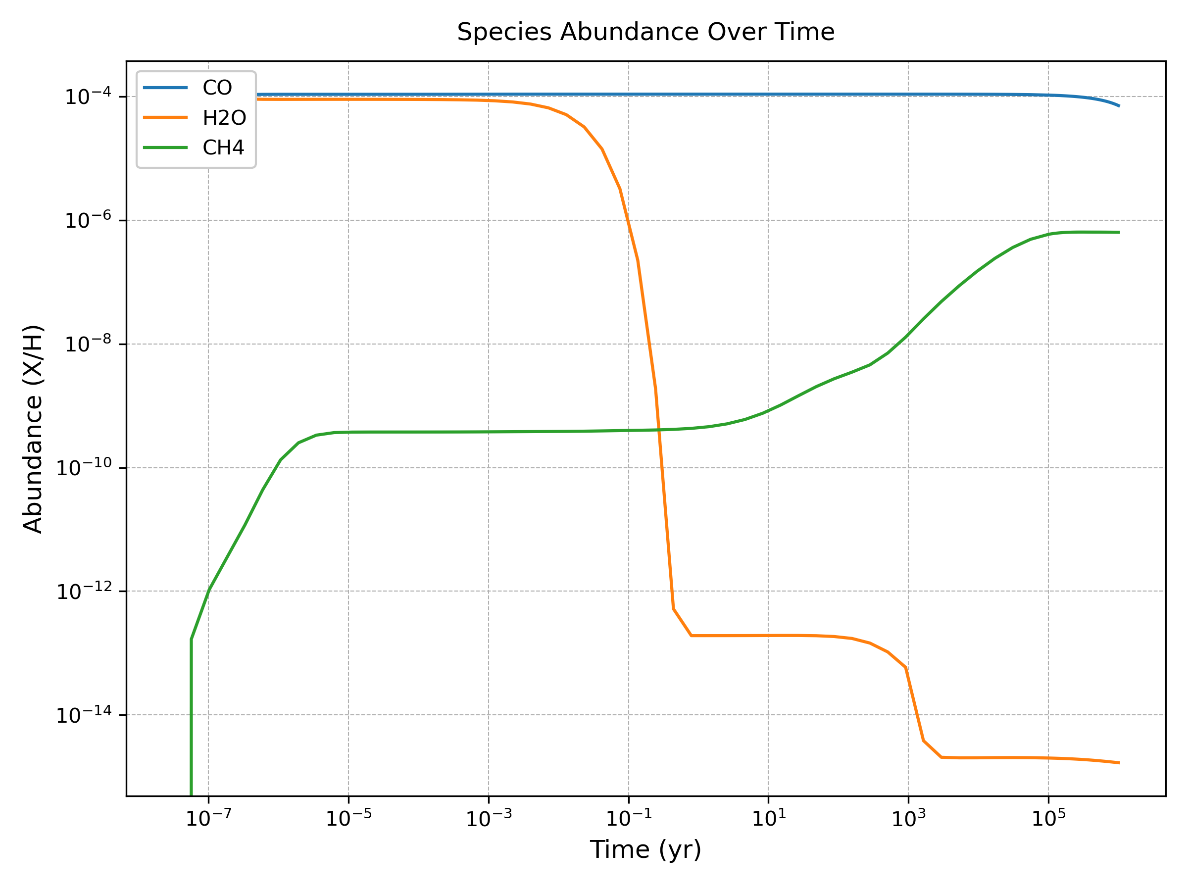
Model outputs (abundances, reaction rates etc) can be plotted using functions in the Analysis module, or using your own code. For example, to plot some abundances vs. time:
# Plot some results
analysis = simba.Analysis(network)
analysis.plot_abundance(['CO', 'H2O', 'CH4'], show=True)